Mapping Ahmedabad’s growth from space: an exploratory look at land-cover change, 2016–2026
Reading this carefully
- Shows
- Where the built-up share of the 48 AMC wards grew between 2016 and 2026: mainly in peripheral wards such as Nikol, Vejalpur, Ghatlodia, Ranip, Chandkheda, Chandlodiya and Vastral, while the old city wards stayed close to stable. A Random Forest and a CNN agree on this pattern (correlation 0.71 between their ward-level changes).
- Doesn’t show
- How much the city grew. The two models put the rise in built-up share at about 10 and 19 percentage points. Only 2021 has an accuracy check, and only against ESA WorldCover, which is itself a model output. The pixel-level change maps are mostly classification error, not change on the ground.
- Connected to
- Conversion of open land and cropland at the city edge; the construction cycle, since cleared land reads as bare soil before it reads as built-up; the crop calendar and irrigation, which blur cropland and natural vegetation in a single dry-season composite; and haze and dust differences in uncorrected Level-1C imagery. None of these were tested in this work.
What this is and why I did it
This is an exploratory analysis of how land cover changed across the 48 wards of the Ahmedabad Municipal Corporation between 2016, 2021 and 2026, using free Sentinel-2 imagery and two machine learning models. The short answer is that both models agree on where the city grew, mainly in the peripheral wards, but they disagree on how much, and with the checks I have done so far the amounts cannot be defended.
I started this as a skill exercise. I wanted to understand what a convolutional neural network (CNN) actually adds over a Random Forest for land-cover mapping, since the usual claim is that deep learning is better but the reason is not always clear. Once that comparison was done it felt natural to push it one step further and ask a real question with it, which was how Ahmedabad has changed over the last ten years.
I am writing this up in some detail because the gap between a convincing map and a reliable one is easy to miss. Most of this article is about how the work was done and where it falls short, and less about the headline numbers. If you are doing similar work, the sections on what is not reliable and on what research-grade work would need are probably the most useful part.
Data: study area, imagery and labels
The study area is the 48 AMC wards. I downloaded the imagery for the wards’ bounding box with a buffer of about 500 m, so that the CNN had some surrounding context at the edges, and then restricted all maps and statistics to the wards themselves.
For each of the three years I made a median composite of Sentinel-2 scenes from 1 March to 30 April in Google Earth Engine. March and April were chosen because it is the dry season in Ahmedabad, so there are few clouds, and the comparison is between the same season every year. Scenes with more than 30% cloud were dropped, and clouds in the remaining scenes were masked using the s2cloudless cloud probability layer (pixels above 40% probability removed). I used six bands (blue, green, red, near infrared and the two shortwave infrared bands) at 10 m, and added three indices: NDVI, MNDWI and NDBI.
The choice of processing level needs a little explanation. The atmospherically corrected product (Level-2A, surface reflectance) is what one would normally use, but in Earth Engine it is not available for India in 2016. Using Level-2A for 2021 and 2026 and the uncorrected Level-1C for 2016 would mean part of any 2016 to 2021 change comes from the different processing and not from the ground. So I used Level-1C (top-of-atmosphere reflectance) for all three years, accepting that haze and dust differences between years are not corrected, in exchange for treating every year the same way. 2016 has another weakness: only Sentinel-2A was in orbit then, so the 2016 composite is built from fewer scenes.
For training labels I used ESA WorldCover v200, a global 10 m land-cover map for 2021. I merged its classes into five: water, built-up, vegetation (trees, shrubs, grassland and mangroves), cropland and bare soil. A few classes that did not fit cleanly, such as herbaceous wetland, were left out of training. Since WorldCover represents 2021, the models were trained only on the 2021 composite. This matters later, because it means accuracy can only be checked for 2021, and only against WorldCover, which is itself a model output and not ground truth.
Two models: Random Forest and a small CNN
The two models look at the image differently. The Random Forest (300 trees) classifies each pixel only from that pixel’s own nine values (six bands and three indices). The CNN is given a 15 × 15 pixel patch, about 150 m across, centred on the pixel, so it can also use the texture and pattern around it. The CNN is deliberately small: three convolution layers, trained for 20 epochs. The idea was to compare the two approaches, not to build the best possible network.
The way the data is split for training and testing turned out to be as important as the models. If training and test pixels are picked at random from the whole image, many test pixels have a training pixel right next to them, and since neighbouring pixels are very similar, the accuracy comes out higher than it should. To avoid this I divided the image into blocks of 2.56 km × 2.56 km and assigned whole blocks to either training (70%) or testing (30%). For the CNN, a pixel was only used if its full patch fell inside one block, so no test patch shares pixels with a training patch. Both models were trained and tested on exactly the same pixels, 2,000 per class for training and 1,000 per class for testing.
Before the multi-year work I ran this comparison once on a single 2024 dry-season scene (Level-2A). The CNN agreed with WorldCover on 70.7% of test pixels and the Random Forest on 60.9%. I repeated it with three different block splits to see whether that gap was luck, and the CNN came out ahead every time, by 9.0 to 9.3 percentage points. The gain was not spread evenly. The CNN was much better at bare soil (76% of bare soil pixels correctly identified against 52%), built-up (72% against 59%) and cropland (69% against 53%), but worse at vegetation (40% against 48%). Built-up areas and bare ground look quite similar spectrally in a dry landscape like Ahmedabad’s, and the most likely reason the CNN separates them better is that it can see the texture of roads and buildings around a pixel. The same context probably hurts with small or scattered vegetation, like a single tree along a road, because a 150 m patch around it is mostly something else.
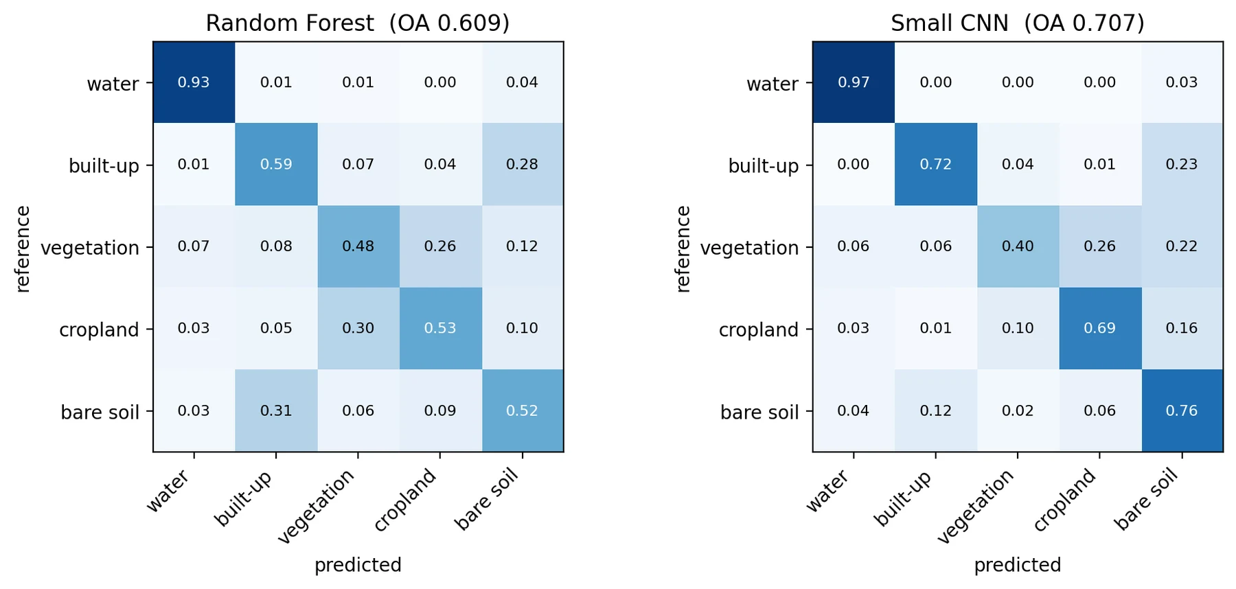
I also checked how much the block split mattered by running the Random Forest once with a random split. The difference was small, 62.2% against 60.9%. I had expected a bigger gap. My understanding is that the leakage was small here because the training pixels were sparse, scattered across a large image, so test pixels rarely sat next to training pixels. With clustered labels, like hand-drawn polygons, the effect would likely be much larger, but I have not tested that.
For the multi-year work both models were retrained on the 2021 Level-1C composite with the same setup. On the held-out 2021 blocks the CNN agreed with WorldCover on 77% of pixels and the Random Forest on 73%. Both numbers are higher than in the 2024 test, but the area, the processing level and the match between image year and label year all changed at once, so I cannot say which of these caused it.
Applying the models to 2016 and 2026
The 2021-trained models were then used to classify every pixel inside the wards for all three years. All three composites were aligned to the same 10 m grid, so a given pixel is the same place on the ground in every year. This step assumes that a model trained on 2021 still works on 2016 and 2026 images, which is reasonable for the same sensor and season but not guaranteed, especially with uncorrected Level-1C data. There are no reference labels for 2016 or 2026, so how well it works for those years is simply not known.
To compare years I did two things. The first was a pixel-by-pixel comparison for three pairs (2016 to 2021, 2021 to 2026 and 2016 to 2026), recording which class each pixel changed from and to. The second was a ward-level summary: for each ward, year and model, the share of the ward’s area in each class. Only pixels that had valid data in all three years were used, so the comparison is always between the same set of pixels.
I expected the ward summaries to be more useful than the pixel comparison. Each map is roughly 70 to 77% accurate, so when two maps are compared pixel by pixel, the errors of both maps show up as change. Averaging over a ward does not remove systematic errors, but it does smooth out a lot of the random ones.
Preliminary results
Both models show the built-up share of the wards increasing over the ten years, but by quite different amounts. The table below gives the city-wide built-up share (by area, across all 48 wards) and how often the two models gave the same class to a pixel.
| Year | Built-up share, Random Forest (%) | Built-up share, CNN (%) | Pixels where RF and CNN agree (%) |
|---|---|---|---|
| 2016 | 37.2 | 35.9 | 60.7 |
| 2021 | 44.7 | 46.9 | 69.6 |
| 2026 | 47.5 | 54.7 | 70.0 |
Over the full period the CNN shows a rise of about 19 percentage points and the Random Forest about 10. Both models agree that the increase from 2016 to 2021 was larger than from 2021 to 2026. That could mean growth slowed, but it could just as well come from the 2016 maps being less reliable, so I would not read anything into it yet.
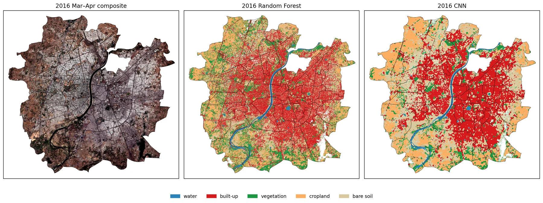
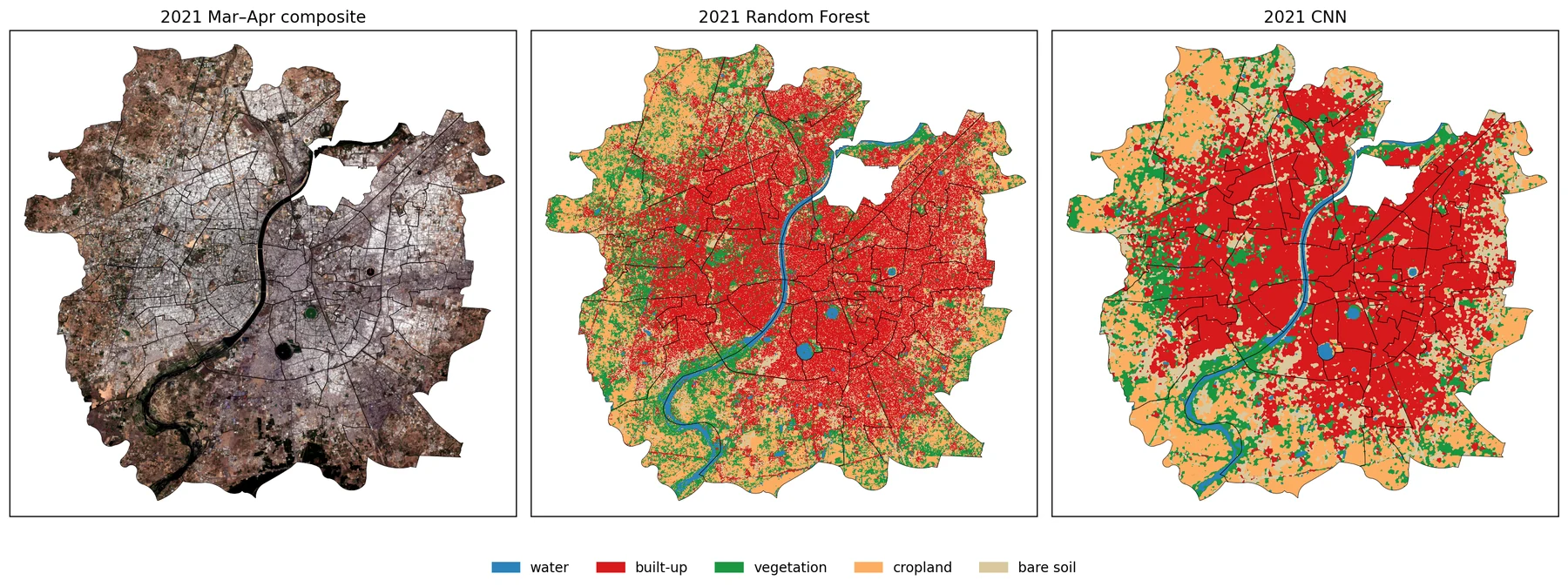
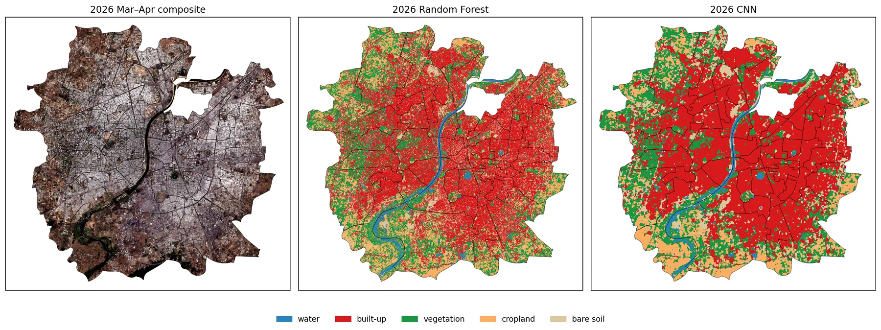
March–April composites and the land-cover maps from both models for 2016, 2021 and 2026 (top to bottom). 2021 is the year the models were trained on and the only year with an accuracy check, so it is the reference for the other two. The Random Forest maps are noticeably more speckled than the CNN maps.
The agreement column is not accuracy, but it is still informative. Two models built differently that give the same answer are more likely to be right than either one alone. Agreement is about 70% in 2021 and 2026 and drops to 61% in 2016, which is the year with the fewest scenes and the most different-looking composite. This is the clearest sign that the 2016 maps are the weakest.
The ward numbers on the map below follow the AMC ward numbering. The table under it gives the name of every ward by its number. The wards discussed in this article are in bold.
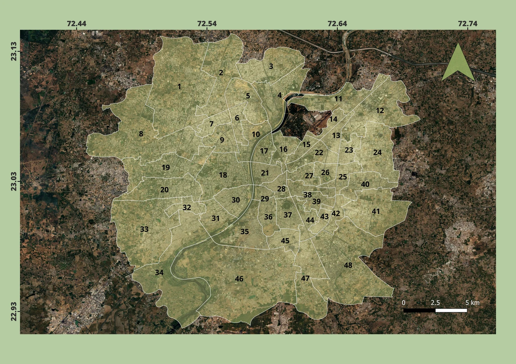
| No. | Ward | No. | Ward | No. | Ward | No. | Ward |
|---|---|---|---|---|---|---|---|
| 1 | Gota | 13 | Saijpur Bogha | 25 | Virat Nagar | 37 | Mani Nagar |
| 2 | Chandlodiya | 14 | Kuber Nagar | 26 | Bapu Nagar | 38 | Gomtipur |
| 3 | Chandkheda | 15 | Asarwa | 27 | Saraspur-Rakhiyal | 39 | Amraiwadi |
| 4 | Sabarmati | 16 | Shahibag | 28 | Khadia | 40 | Odhav |
| 5 | Ranip | 17 | Shahpur | 29 | Jamalpur | 41 | Vastral |
| 6 | New Wadaj | 18 | Navrangpura | 30 | Paldi | 42 | Indrapuri |
| 7 | Ghatlodia | 19 | Bodakdev | 31 | Vasna | 43 | Bhaipura Hatkeshwar |
| 8 | Thaltej | 20 | Jodhpur | 32 | Vejalpur | 44 | Khokhra |
| 9 | Naranpura | 21 | Dariyapur | 33 | Sarkhej | 45 | Isanpur |
| 10 | S. P. Stadium | 22 | India colony | 34 | Maktampura | 46 | Lambha |
| 11 | Sardar Nagar | 23 | Thakkarbapa Nagar | 35 | Baherampura | 47 | Vatva |
| 12 | Naroda | 24 | Nikol | 36 | Danilimda | 48 | Ramol Hathijan |
At ward level the two models agree much better on where growth happened than on how much. The largest gains in built-up share from 2016 to 2026 in both models are in peripheral wards such as Nikol, Vejalpur, Ghatlodia, Ranip, Chandkheda, Chandlodiya and Vastral. Across the 48 wards the correlation between the two models’ change values is 0.71, so they rank the wards in a broadly similar way even though the CNN’s changes are generally larger.
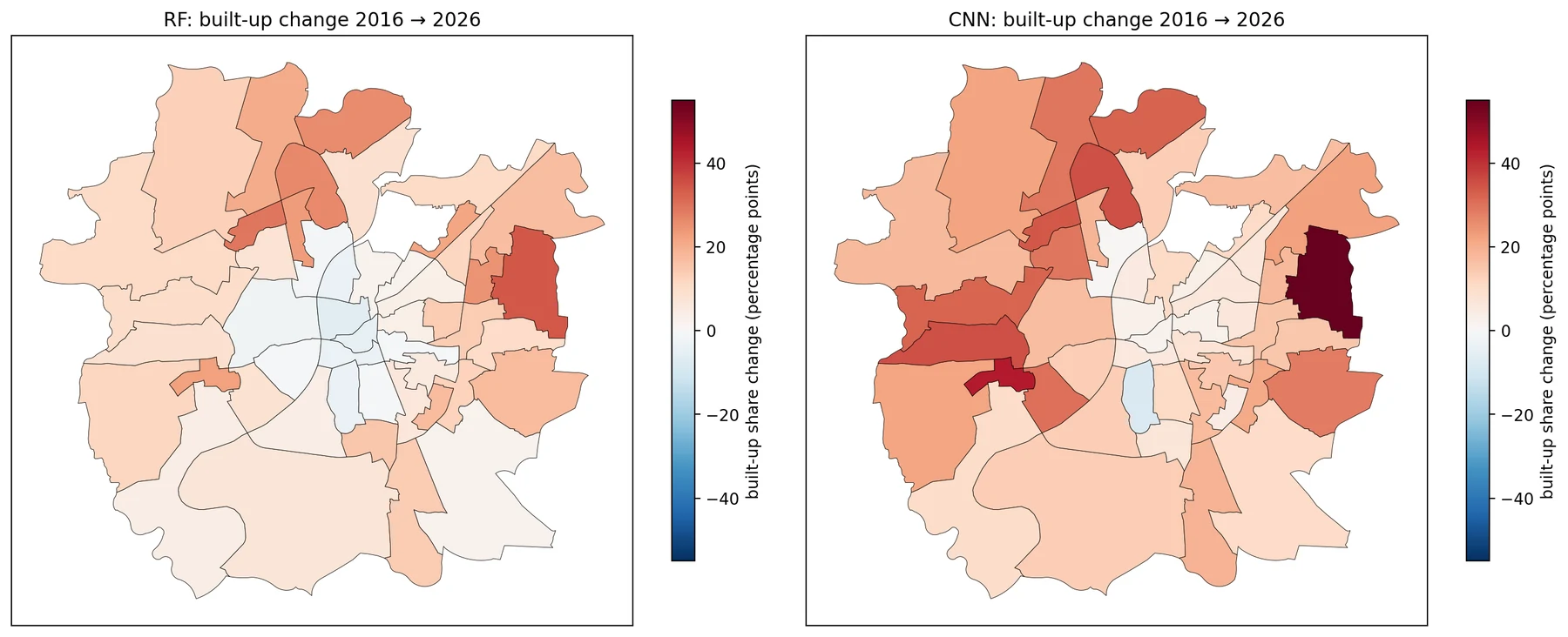
The old city wards (Khadia, Dariyapur, Jamalpur and Shahpur) work as a useful sanity check. These areas have been densely built for centuries, so their built-up share should hardly change. For 2021 to 2026 the CNN shows changes of about 0 to +6 percentage points there, which is plausible. The Random Forest shows drops of 4 to 14 points, which is not, and is most likely noise from per-pixel classification in a dense, mixed urban fabric. This is one more point in favour of the CNN, alongside the 2021 accuracy.
One ward, Danilimda, shows a decrease in built-up share in both models. I have not checked this against high-resolution imagery, so for now it is only something worth looking into.
What is not real, or not reliable
The pixel-level change maps are the clearest example. Between 2016 and 2026 the CNN shows 47% of ward pixels changing class and the Random Forest 51%; even the five-year pairs show 30 to 44%. No city changes half its surface in ten years, so most of this is the combined error of two maps. The Random Forest maps are also visibly speckled (salt-and-pepper noise), which adds to the false change. These maps look dramatic, and that is exactly why they should not be read as results.
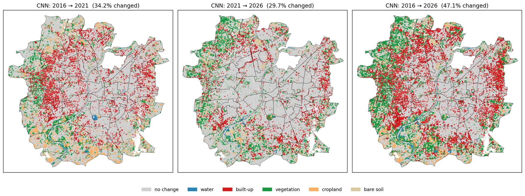
The largest single transition, bare soil to built-up (about 80 km² in the CNN and 56 km² in the Random Forest from 2016 to 2026), needs care for a different reason. Some of it is surely real, since construction on open land is how a city grows. But built-up and bare soil is also the pair the models confuse most, as the earlier comparison showed. So part of this transition is the classifier and not construction, and I have no way yet to separate the two. In the CNN the bare soil share falls from about 33% in 2016 to about 10% in 2026, which is more than I would believe without checking.
Cropland turning into vegetation (around 33 to 36 km² in both models) is most likely not land-use change at all. In March and April some fields have been harvested, some are irrigated and green, and the timing changes from year to year. A green field and natural vegetation can look much the same in a single-season composite. With only one season per year, these two classes are not stable enough to compare across years.
Finally, the 2016 maps are weaker than the others for the reasons already mentioned: fewer scenes, no atmospheric correction and the lowest agreement between the models. Some of the 2016 to 2021 change is probably a difference in how the images look rather than in what is on the ground.
What it would take to make this research-grade
What I have now supports one claim: the spatial pattern of where Ahmedabad’s built-up area grew between 2016 and 2026, with the periphery growing and the old city stable. Two different models agree on it and it passes the old city check. The amounts of change, in km² or percentage points, are not supported, and I would not quote them as findings.
To get from here to something defensible, the most important missing piece is an independent accuracy assessment for every year. That would mean a stratified random sample of points, something like 50 or more per class per year, each checked by eye against historical high-resolution imagery such as Google Earth. From that, the accuracy of each map can be estimated, and the class areas can be corrected for known errors, with confidence intervals, rather than taken straight from pixel counts. Without this, there is no basis for saying how much of the change is real.
A few other changes would help. The class definitions should be ones that stay stable across years: merging vegetation and cropland into a single green or agricultural class, for example, would remove the seasonal problem described above. Using imagery from more than one season, or a time series within each year, would help separate crops from natural vegetation if that distinction is needed. The 2016 data problem could be handled either by doing an atmospheric correction myself or by using Landsat 8, which has surface reflectance for 2016, at the cost of 30 m resolution. And the change estimates themselves should come with uncertainty, so that a ward’s change can be judged against the error rather than read as a single number.
None of this is unusual. It is standard practice in land-cover change studies, and it is also the part that takes most of the time. That is the main difference between this exploratory version and a research version: not a better model, but a proper way of knowing how wrong the maps are.
What I learned
On the modelling side, the CNN’s advantage was real and consistent, about 9 points in the single-scene test and 4 points on 2021, and it came mostly from classes that are spectrally similar but differ in texture. It was not better at everything, and it was worse at small, scattered vegetation. The old city check was a cheap way to catch a problem that the accuracy numbers alone did not show.
On the method side, the spatial split mattered less than I expected in this setup, and I now think the reason is the sparse sampling rather than the split being unimportant. Repeating the comparison with three different splits was worth the extra run time, because the single-run gap turned out to be slightly overstated. And the multi-year part made it very clear that a map that looks convincing and a change estimate that can be defended are two different things. Most of the effort in real work would go into the second.
Method
- Data
- Sentinel-2 Level-1C (top-of-atmosphere reflectance) with the s2cloudless cloud probability layer, 1 March–30 April of 2016, 2021 and 2026; a single 2024 Level-2A dry-season scene for the model comparison; ESA WorldCover v200 (2021) for training labels; AMC ward boundaries (shapefile)
- Processing
- Median composites in Google Earth Engine through geemap; scenes over 30% cloud dropped and pixels above 40% cloud probability masked; six 10 m bands plus NDVI, MNDWI and NDBI; all years on one 10 m grid
- Models
- Random Forest (300 trees, scikit-learn) on per-pixel values; a three-layer CNN (PyTorch, 20 epochs) on 15 × 15 pixel patches; spatial block split of 2.56 km blocks, 70% training and 30% testing, 2,000 training and 1,000 test pixels per class
- Checks
- Agreement with WorldCover on held-out 2021 blocks; three repeated block splits; a random-split comparison; agreement between the two models; the old city stability check. No independent accuracy assessment for any year
- Code
- Two Jupyter notebooks (model comparison; multi-year ward analysis). Available on request.
A question for readers
If you spot a mistake or have done something similar for another city, I would like to hear about it.